Why 3× Daily Leverage Is Not 3× Long-Term Return

A quantitative look at daily reset, compounding, path dependence, volatility and real leveraged ETF data, with a reproducible notebook.

---

A 3× leveraged ETF sounds simple: if the underlying index goes up by 1%, the fund should go up by about 3%. So if the index gains 20% over a year, shouldn’t the leveraged fund gain about 60%?

Not necessarily.

The reason is hidden in one word that is easy to overlook: daily.

A daily 3× leveraged ETF aims to deliver roughly three times the index’s return each day. For example, ProShares currently states that TQQQ seeks three times the daily performance of the Nasdaq-100 Index, before fees and expenses. Once those daily returns are compounded over many days, the result depends not only on where the index finishes, but also on the path it took to get there.

That difference is not a minor technicality. It is one of the central mathematical features of leveraged ETFs.

This article grew out of two LinkedIn posts in which I explored the mechanism using simple examples, code and real market data. It also connects to a supervised research project on leveraged ETF performance that I later advised at SCE.

Start with an ordinary investment

Suppose an asset falls by 10%.

An investment of 100 becomes 90.

How much does it need to rise to return to 100?

Not 10%.

A 10% increase from 90 only gets us to 99. To return from 90 to 100, the required gain is

$$\frac{100}{90}-1 \approx 11.11\%.$$

This asymmetry is a basic consequence of compounding: a percentage loss and an equal percentage gain do not cancel each other because the second percentage is applied to a different base.

More generally, if an asset falls by a fraction $x$, then the gain required to recover exactly is

$$\frac{x}{1-x}.$$

For $x=0.10$, this gives $0.10/0.90 = 0.1111$, or 11.11%.

Now apply daily leverage

Consider an idealized 3× daily leveraged product.

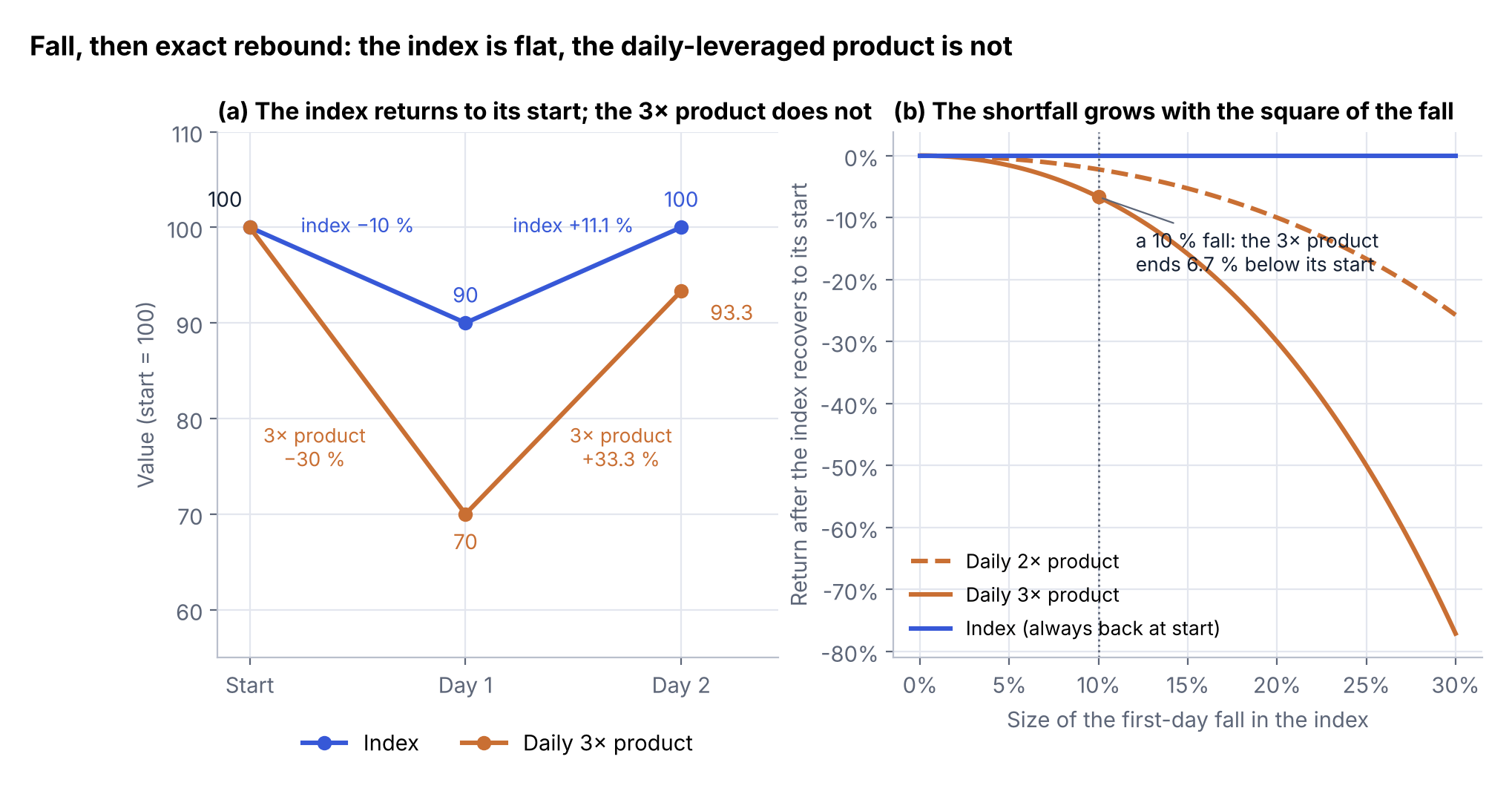
If the underlying falls 10% on day 1, the leveraged product falls approximately 30%:

$$100 \rightarrow 70.$$

On day 2, suppose the underlying rises 11.11%, exactly enough to recover its original value.

A 3× daily product would then gain approximately 33.33% on that day:

$$70 \times 1.3333 \approx 93.33.$$

The underlying is back where it started.

The leveraged product is down about 6.67%.

This is the first important lesson:

A leveraged ETF multiplies each day’s return. It does not simply multiply the final multi-day return.

Mathematical insight

The same example in one formula

The result above can be written more generally.

Suppose the underlying first falls by $x$, then rises by exactly the amount required to return to its initial value:

$$(1-x)\left(1+\frac{x}{1-x}\right)=1.$$

For an idealized daily leveraged product with leverage factor $L$, the two-day value becomes

$$(1-Lx)\left(1+L\frac{x}{1-x}\right).$$

After simplification,

$$V_2^{(L)} = 1-\frac{L(L-1)x^2}{1-x}.$$

So whenever $L>1$ and the leveraged product remains mathematically feasible over the move, this particular down-then-recovery path leaves the leveraged position below its starting value.

For $L=3$ and $x=0.10$,

$$1-\frac{3(2)(0.1)^2}{0.9} = 0.9333.$$

That is the same 6.67% loss we obtained numerically.

The formula also reveals something that the numerical example hides: the gap grows approximately with the square of the size of the move. Small fluctuations matter little; large back-and-forth moves matter much more.

A real market example: a dividend-adjusted round trip

The synthetic examples isolate the mathematics. But the same pattern appears in actual market data.

One example I found while exploring this question in a Colab notebook occurred over two close-to-close return intervals in June 2024:

Date	QQQ adjusted	TQQQ adjusted	SQQQ adjusted
June 21, 2024	474.442	36.454	179.868
June 24, 2024	469.041	35.219	186.077
June 25, 2024	474.405	36.395	179.654

From the June 21 close to the June 25 close:

• QQQ’s dividend-adjusted return was approximately −0.008%;
• TQQQ returned approximately −0.161%;
• SQQQ returned approximately −0.119%.

So the benchmark proxy ended essentially flat after accounting for QQQ’s June 24 distribution, while both the daily +3× and −3× products ended slightly below their starting values.

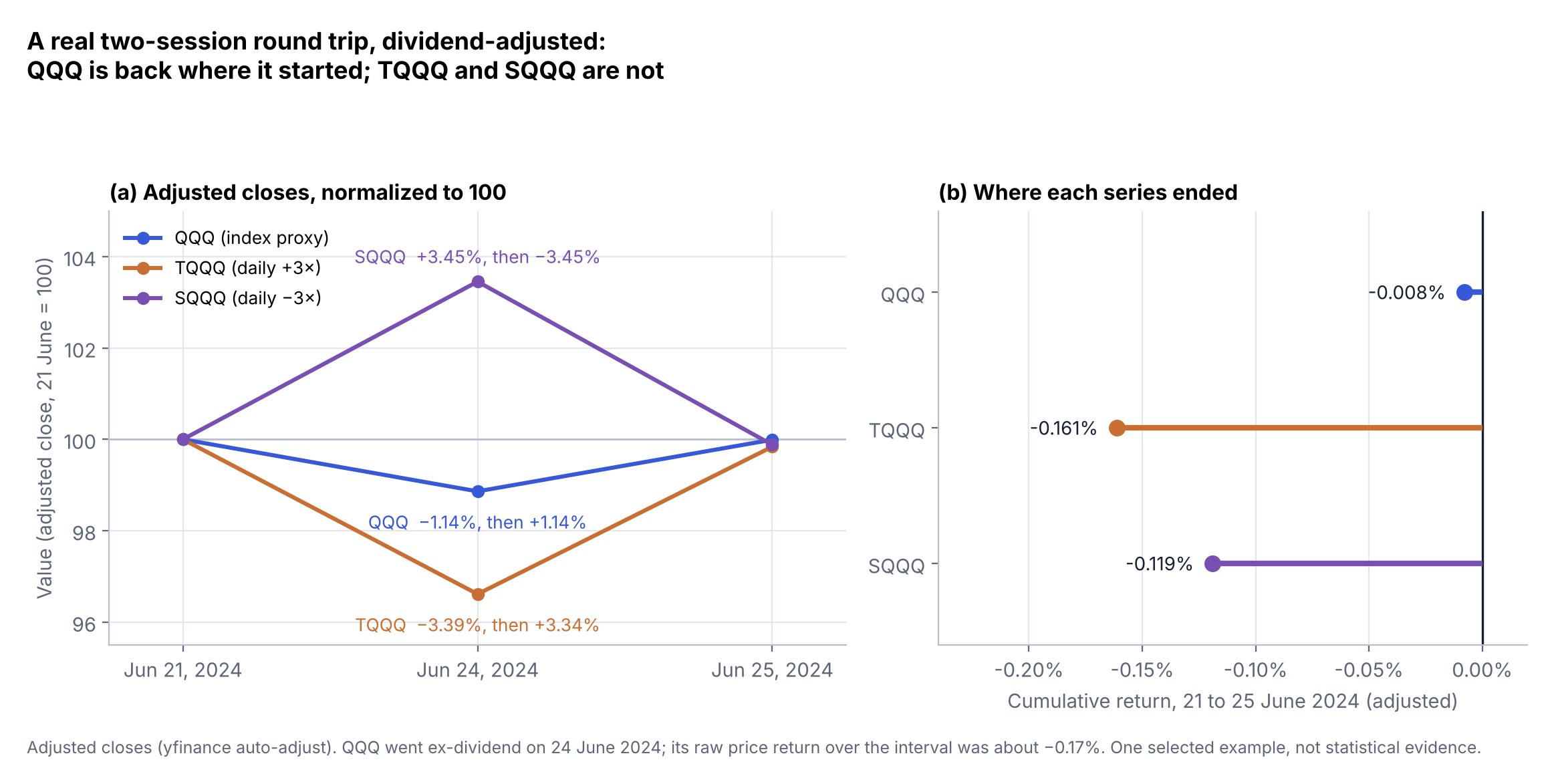
That is exactly the sort of real-world example I wanted to find: not a simulation, but a concrete market realization that readers can check independently. The three-date data snapshot and its source notes are published with the notebook.

There is an important qualification, and checking it was part of the work. After reproducing the example from adjusted prices, I compared it with an independent series of unadjusted closes. That showed that QQQ went ex-dividend on June 24 (a distribution of 0.7615 US dollars per share). On raw closing prices QQQ’s return over the interval is about −0.17%; adding back the distribution gives the −0.008% above. The near-flat result is therefore a dividend-adjusted return statement, not an unadjusted price statement. The independent series also agrees with the TQQQ and SQQQ endpoint returns.

The TQQQ and SQQQ price levels in the table also reflect retrospective split adjustments. That does not materially affect their endpoint returns over this interval, but it is why the adjustment convention is stated explicitly rather than treating the levels as raw prices.

Stated precisely:

From the June 21 close to the June 25 close, QQQ’s dividend-adjusted return was approximately −0.008%, while TQQQ and SQQQ returned approximately −0.161% and −0.119%, respectively.

It is a real-market illustration consistent with the compounding mechanism, but it does not isolate compounding perfectly. Actual ETF returns also include financing, fees, market-price/NAV differences, and tracking effects.

There is another useful comparison. If we take QQQ’s two observed daily returns and apply an idealized daily-reset rule directly to them, we obtain approximately:

• idealized +3× cumulative return: −0.102%;
• idealized −3× cumulative return: −0.132%.

The actual TQQQ and SQQQ returns over the same window were approximately −0.161% and −0.119%, respectively.

The signs are consistent with the compounding mechanism, but the small differences between idealized and observed outcomes should not be over-interpreted. Three dates cannot separate financing, fees, tracking residuals, QQQ-versus-Nasdaq-100 differences, and closing-price effects.

There is also a selection caveat: the original notebook searched historical QQQ data for a loss-and-rebound sequence. This example was therefore selected because it illustrates the mechanism clearly. It is not evidence about how frequently such round trips occur or about the expected performance of leveraged ETFs.

TQQQ and SQQQ contractually target the Nasdaq-100 Index, not QQQ shares themselves. QQQ is used here as a convenient tradable proxy, so this is an illustration of the observed pattern rather than a formal tracking-error calculation.

Mathematical insight

Why the path matters

Now consider daily returns $r_1,r_2,\ldots,r_T$.

An unleveraged investment evolves as

$$V_T = V_0\prod_{t=1}^{T}(1+r_t).$$

An idealized daily $L$-times leveraged investment evolves approximately as

$$V_T^{(L)} = V_0\prod_{t=1}^{T}(1+Lr_t).$$

These expressions look similar, but they are not related by a simple final multiplication.

In general,

$$\prod_{t=1}^{T}(1+Lr_t) \neq 1+L\left(\prod_{t=1}^{T}(1+r_t)-1\right).$$

Nor is it generally true that

$$\prod_{t=1}^{T}(1+Lr_t) = \left(\prod_{t=1}^{T}(1+r_t)\right)^L.$$

The size and composition of the daily moves matter because the leveraged product compounds each reset-period return separately.

This property is usually described as path dependence: knowing only the benchmark’s starting value and ending value is not enough to determine what happened to the leveraged product.

There is an important precision here. In the ideal fixed-leverage model, simply reordering the exact same set of daily returns does not change terminal wealth, because multiplication is commutative. What matters is that many different collections of daily returns can lead the benchmark to the same final value while producing different leveraged outcomes.

Two paths can end at the same place and still produce different leveraged outcomes

A particularly clean way to see path dependence is to compare two paths with exactly the same underlying endpoint.

Path A: relatively smooth

Suppose the underlying gains 5% on each of two days:

$$1.05\times1.05=1.1025.$$

The two-day return is 10.25%.

An idealized 3× daily product experiences +15% and +15%:

$$1.15\times1.15=1.3225.$$

Its two-day return is 32.25%.

Path B: much more volatile

Now suppose the underlying first falls 10%, then rises 22.5%:

$$0.90\times1.225=1.1025.$$

The underlying again finishes with exactly the same 10.25% two-day return.

But the idealized 3× product now experiences -30% followed by +67.5%:

$$0.70\times1.675=1.1725.$$

Its return is only 17.25%.

Same underlying starting value. Same underlying ending value. Very different leveraged result.

That is path dependence in its most concrete form.

The difference comes from repeatedly multiplying each day’s leveraged growth factor, $1+Lr_t$, along the path. The final index return alone therefore cannot determine the long-horizon return of a daily-reset leveraged product.

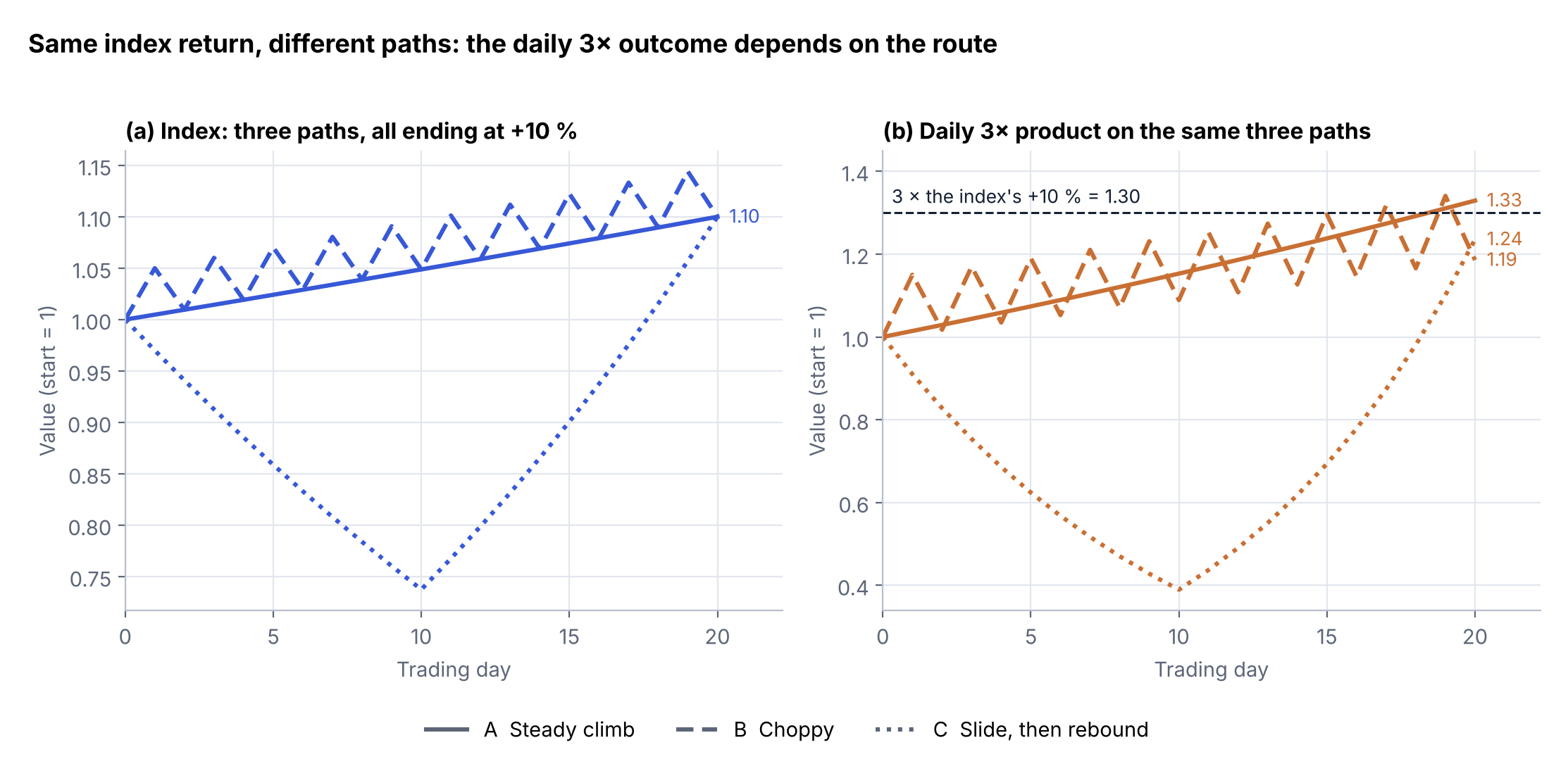
The same idea at a longer horizon: take three 20-day index paths that all end at exactly +10%. In the idealized model, a steady climb leaves a daily 3× product at about 1.33 times its start, a slide followed by a rebound at about 1.24 times, and a choppy path at about 1.19 times, compared with 1.30 for “three times the index’s gain”.

Mathematical insight

Where “volatility drag” comes from

A useful way to see the effect is through logarithms.

For a small daily return $r$,

$$\log(1+r) \approx r-\frac{r^2}{2}.$$

For an idealized $L$-times daily return,

$$\log(1+Lr) \approx Lr-\frac{L^2r^2}{2}.$$

Now compare that with simply taking $L$ times the unleveraged log return:

$$L\log(1+r) \approx Lr-\frac{Lr^2}{2}.$$

The difference is approximately

$$-\frac{L(L-1)}{2}r^2.$$

Because $r^2$ is always non-negative, back-and-forth variation creates a compounding penalty relative to the naive idea of “just multiply the long-term return by $L$.”

Across many days, this quadratic term accumulates.

This is one mathematical way to understand what is commonly called volatility drag, variance drag, or volatility decay.

Those labels are useful only if we say exactly what is being compared. Two related quantities are often mixed together:

• the negative variance contribution to logarithmic growth;
• the signed difference between the leveraged product’s cumulative return and a naïve benchmark such as $L$ times the benchmark’s cumulative return.

The first is a genuine variance penalty in the growth-rate approximation. The second can be called compounding deviation only when we are comparing the ideal daily-compounded leveraged return with $L$ times the benchmark’s cumulative return. For an actual ETF, the observed difference also contains financing, fees, tracking, and other implementation effects, so it is better described as a total return deviation from the naïve multiple.

So volatility does not imply that a leveraged ETF must lose money, and leverage does not imply inevitable decay. A sufficiently strong positive drift can more than compensate for the variance penalty.

A more precise summary is:

Variance penalizes geometric growth, and leverage magnifies that penalty, but the total long-horizon outcome also depends on drift, funding, fees, and the realized return path.

A strong, persistent trend can push in the other direction. For example, two +10% days produce a benchmark return of 21%, while an idealized daily 3× product returns 69%, which is more than the naïve 63% obtained by tripling the benchmark’s two-day return. Daily compounding therefore does not create a one-way “decay”; it changes the result in a path-dependent way.

From average returns to compounded wealth

Another source of confusion is the difference between the arithmetic average return and the growth of wealth.

Suppose returns alternate between +10% and -10%.

Their arithmetic average is 0%.

But wealth evolves as

$$1.10\times0.90 = 0.99.$$

So the investor loses 1%.

The average return is zero, but the compounded return is negative.

This is why geometric growth matters whenever returns are repeatedly multiplied through time.

The publication notebook makes the same point with reproducible simulations. It holds the arithmetic drift fixed, varies volatility, and compares both the typical outcome and the full distribution for 1× and idealized 3× exposure.

What changes when volatility changes?

A historical example is useful because it is real; a simulation is useful because it lets us control the mechanism. Holding arithmetic drift fixed while changing volatility allows us to see how much of the outcome comes from the interaction between leverage and compounded variation.

In the simulations below, daily returns are drawn independently from a normal distribution with an arithmetic drift of 8% a year, volatility between 10% and 60% a year, five years of trading days, and no fees or financing. The 8% drift is a deliberate illustrative boundary case, not a calibration to any market.

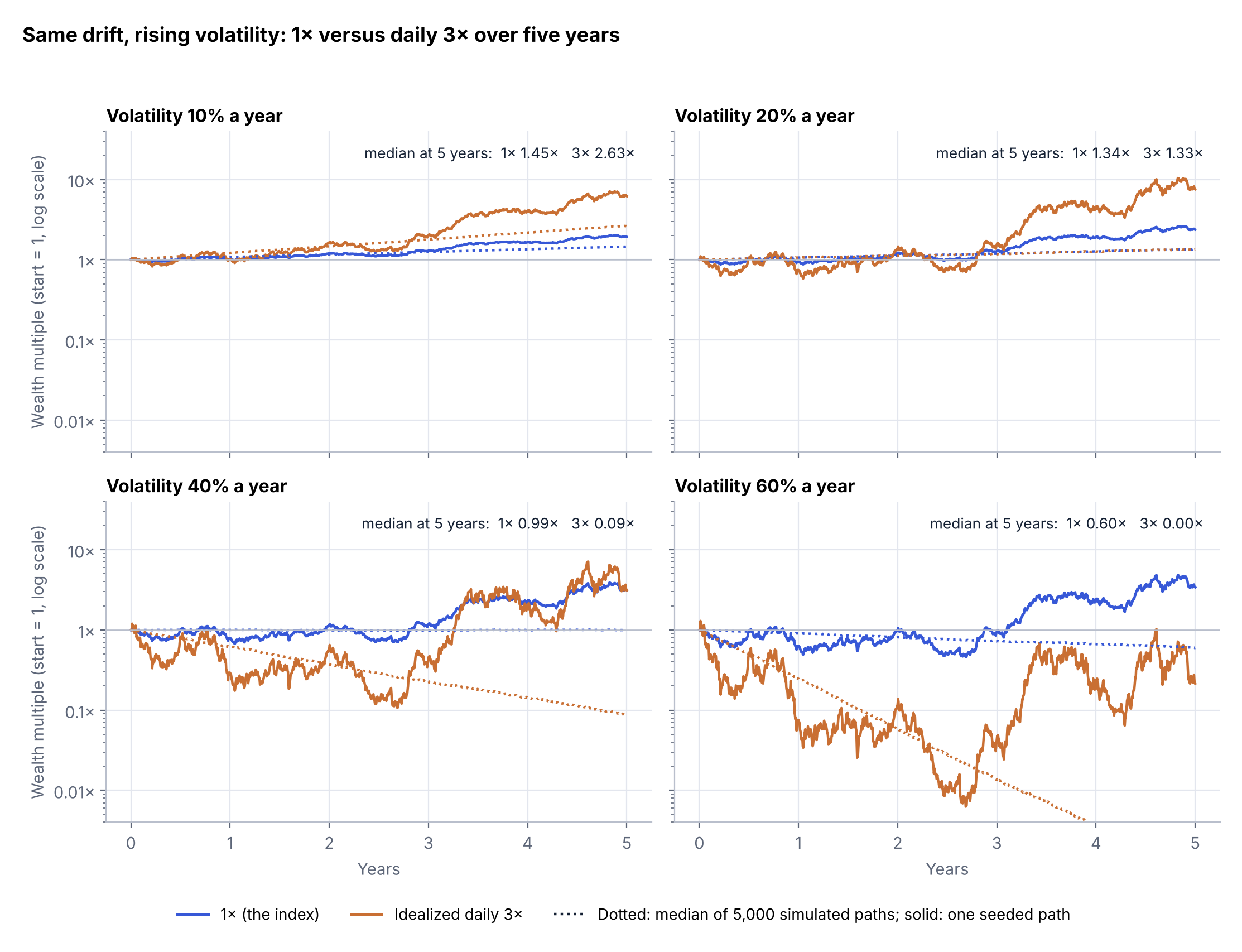
In numbers, the median five-year outcome at 10% volatility is about 2.6 times the starting value for the 3× product against 1.45 for the index. At 20% the medians are about equal (1.34 and 1.33). At 40% the median 3× path ends near 0.09 times its start while the index ends near 0.99.

The important outputs are not only terminal averages. We also compare medians, quantiles, and the probability that the leveraged product finishes below the unleveraged path. The goal is not to forecast a particular ETF, but to isolate the mathematics.

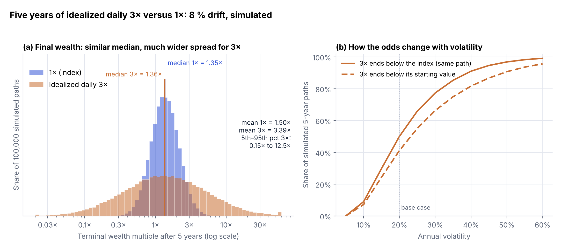
At 20% volatility (100,000 simulated paths) the medians are about 1.35 times the starting value for the index and 1.36 for the 3× product, but the means are about 1.5 and 3.4. The 3× product ends below its starting value in about 41% of paths, against 25% for the index, and its middle 90% of outcomes spans roughly 0.15 to 12.5 times the start. A mean pulled up by rare very large outcomes and a median that describes a typical path are answering different questions.

From a simple LinkedIn example to a supervised empirical study

The same question later appeared in a student research project I supervised at SCE: Stability of Leveraged ETF Performance, by Daniel Shub and Pavel Zaikin.

The project studied 18 leveraged ETFs matched with 16 benchmarks. Using nine annual entry dates and both variable and fixed one-year holding periods, it produced 324 entry cases designed to measure how strongly outcomes change across starting points and volatility regimes, not to identify a “best” entry date.

Read the supervised project →

The project is a useful empirical companion to the mathematical explanation here. This article explains the mechanism. The project asks how strongly that mechanism appears across historical windows and instruments.

Real leveraged ETFs are more complicated than the idealized equations

The equations above describe an idealized product that delivers exactly $L$ times the underlying’s daily return.

Real funds have additional layers:

• management fees;
• financing costs;
• derivatives and collateral;
• trading and rebalancing frictions;
• tracking error;
• fund-specific constraints;
• extreme-market effects.

These effects can widen the gap between the idealized leveraged path and an actual ETF. The compounding mechanism exists even before they are introduced, but real investor outcomes reflect both the mathematics of daily reset and the implementation of the fund.

So are leveraged ETFs unsuitable for long-term holding?

That question is too broad to answer with a slogan.

The long-horizon outcome depends on several interacting quantities:

• the underlying asset’s drift, meaning its average directional tendency;
• volatility;
• the leverage factor;
• the sequence of returns;
• the holding period;
• fees and financing;
• tracking quality;
• the structure of the product.

A leveraged ETF can dramatically outperform its unleveraged benchmark over some long periods and dramatically underperform it over others. The useful conclusion is narrower:

Daily leverage is a rule applied to daily returns. Long-term performance emerges from compounding those returns, not from multiplying the benchmark’s final cumulative return by the leverage factor.

Once that distinction is clear, both the opportunity and the risk become easier to analyze quantitatively.

Practical takeaway

If you see “3×” in the name of a daily-reset leveraged ETF, the safest mental translation is:

approximately three times the benchmark’s daily return

not:

three times whatever the benchmark earns over my whole holding period.

Those are fundamentally different claims. The first is the product objective; the second is generally false.

Further reading

A short technical bibliography for this article:

• Marco Avellaneda and Stanley Zhang (2010), “Path-Dependence of Leveraged ETF Returns,” SIAM Journal on Financial Mathematics (DOI 10.1137/090760805). The main mathematical reference for the long-horizon path and variance identity.
• Robert A. Jarrow (2010), “Understanding the Risk of Leveraged ETFs,” Finance Research Letters (DOI 10.1016/j.frl.2010.04.001). Useful for the dynamic-replication and financing interpretation.
• Hongfei Tang and Xiaoqing Eleanor Xu (2013), “Solving the Return Deviation Conundrum of Leveraged Exchange-Traded Funds,” Journal of Financial and Quantitative Analysis (DOI 10.1017/S0022109012000622). Particularly useful for separating compounding deviation from tracking and implementation deviation.
• Narat Charupat and Peter Miu (2014), “A New Method to Measure the Performance of Leveraged Exchange-Traded Funds,” The Financial Review (DOI 10.1111/fire.12055). An empirical decomposition into compounding, financing and management effects.
• U.S. Securities and Exchange Commission, Office of Investor Education and Advocacy (2023), “Updated Investor Bulletin: Leveraged and Inverse ETFs.” A regulatory explanation of the daily objective and of the risks of reading it over longer horizons.
• ProShares, TQQQ product page (accessed October 7, 2026), and the TQQQ Summary Prospectus dated September 26, 2025, with the February 18, 2026 supplement. The product page states the daily objective and the longer-horizon warning; the dated prospectus defines the objective on a NAV-to-NAV basis.

For broader mathematical background, Robert C. Merton’s continuous-time portfolio model (1969) and John L. Kelly Jr.’s growth criterion (1956) help explain why expected wealth, median wealth and logarithmic growth answer different questions.

Related work on this site

• Stability of Leveraged ETF Performance: the empirical companion to this article, a supervised study of 18 leveraged ETFs across 324 entry cases.
• Data-Driven Risk-Adjusted Performance Analysis: a regime-aware comparison of classical risk-adjusted ratios with a structural exponential-fit score, also presented at ADTM 2026.
• TradeMind: a supervised platform that models market states probabilistically and turns the forecasts into risk-aware analysis.

Provenance

This article expands a series of LinkedIn posts:

• July 2, 2026: leveraged ETFs, recovery after a loss, and daily compounding (post)
• June 29, 2025: why 3× daily leverage does not imply 3× long-term return (post)

Interested in quantitative research, modeling or applied statistical problems? Get in touch.